Series: Python for kids
In our endavor to make learning fun and free of memorization, we have been using Python to allow children to experiment and analyze data to form their own opinion and discover facts. This way, children engage is learning process with more intensity and the they show higher retention rate vis a vis conventional learning.
This makes them think and try different things before they get it right. The focus shifts from being always ‘right’ to get it right after several failed attempts.
In this part of the series
Children create simple shapes using markers, move marker left, right , top and bottom. They learn coordinates geometry where the position of points on the plane.
In this blog we are using Matplotlibn library. Matplotlib is a plotting library for the Python programming language and its numerical mathematics extension NumPy.
import matplotlib.pyplot as plt
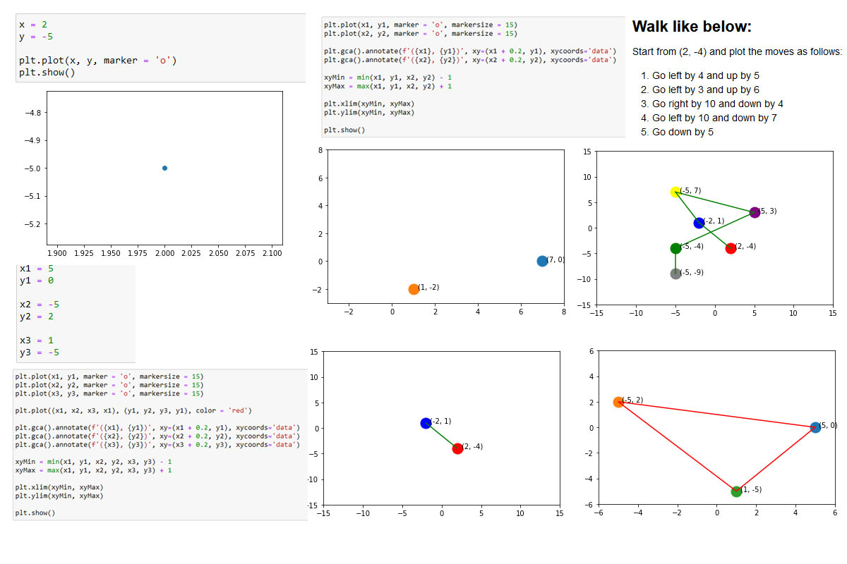
x = 2
y = -5

plt.plot(x, y, marker = 'o')
plt.show()

plt.plot(x, y, marker = 'o', markersize = 15)
plt.show()

matplotlib.pyplot.xlim(*args, **kwargs): Get or set the x limits of the current axes.
matplotlib.pyplot.ylim(*args, **kwargs): Get or set the y limits of the current axes.
We are getting min and max of x and y value, after that setting the limits of X-axis between min and max value. Same thing we are doing to set Y-axis limit.
plt.plot(x, y, marker = 'o', markersize = 15)
plt.gca().annotate(f'({x}, {y})', xy=(x + 0.2, y), xycoords='data')

xyMin = min(0, x, 0, y) - 1
xyMax = max(0, x, 0, y) + 1

plt.xlim(xyMin, xyMax)
plt.ylim(xyMin, xyMax)

plt.show()

x1 = 7
y1 = 0

x2 = 1
y2 = -2
plt.plot(x1, y1, marker = 'o', markersize = 15)
plt.plot(x2, y2, marker = 'o', markersize = 15)

xyMin = min(x1, y1, x2, y2) - 1
xyMax = max(x1, y1, x2, y2) + 1

plt.xlim(xyMin, xyMax)
plt.ylim(xyMin, xyMax)

plt.show()

plt.plot(x1, y1, marker = 'o', markersize = 15)
plt.plot(x2, y2, marker = 'o', markersize = 15)

plt.gca().annotate(f'({x1}, {y1})', xy=(x1 + 0.2, y1), xycoords='data')
plt.gca().annotate(f'({x2}, {y2})', xy=(x2 + 0.2, y2), xycoords='data')

xyMin = min(x1, y1, x2, y2) - 1
xyMax = max(x1, y1, x2, y2) + 1

plt.xlim(xyMin, xyMax)
plt.ylim(xyMin, xyMax)

plt.show()

x1 = 5
y1 = 0

x2 = -5
y2 = 2

x3 = 1
y3 = -5
plt.plot(x1, y1, marker = 'o', markersize = 15)
plt.plot(x2, y2, marker = 'o', markersize = 15)
plt.plot(x3, y3, marker = 'o', markersize = 15)

plt.plot((x1, x2, x3, x1), (y1, y2, y3, y1), color = 'red')

plt.gca().annotate(f'({x1}, {y1})', xy=(x1 + 0.2, y1), xycoords='data')
plt.gca().annotate(f'({x2}, {y2})', xy=(x2 + 0.2, y2), xycoords='data')
plt.gca().annotate(f'({x3}, {y3})', xy=(x3 + 0.2, y3), xycoords='data')

xyMin = min(x1, y1, x2, y2, x3, y3) - 1
xyMax = max(x1, y1, x2, y2, x3, y3) + 1

plt.xlim(xyMin, xyMax)
plt.ylim(xyMin, xyMax)

plt.show()

x = 2
y = -4

plt.plot(x, y, marker = 'o', color = 'red', markersize = 10)
plt.gca().annotate(f'({x}, {y})', xy=(x + 0.2, y), xycoords='data')

plt.xlim(-15, 15)
plt.ylim(-15, 15)
plt.show()

x = 2
y = -4

plt.plot(x, y, marker = 'o', color = 'red', markersize = 15)
plt.gca().annotate(f'({x}, {y})', xy=(x + 0.5, y), xycoords='data')

#declare a starting point, which is x and y
xStart = x
yStart = y

#move left by 4, so x will be xstart + (-4)
#move up by 5, so y will be ystart + 5
x = xStart + -4
y = yStart + 5

plt.plot(x, y, marker = 'o', color = 'blue', markersize = 15)
plt.gca().annotate(f'({x}, {y})', xy=(x + 0.5 , y), xycoords='data')
plt.plot((xStart, x), (yStart, y), color = 'green')


plt.xlim(-15, 15)
plt.ylim(-15, 15)
plt.show()

x = 2
y = -4

plt.plot(x, y, marker = 'o', color = 'red', markersize = 15)
plt.gca().annotate(f'({x}, {y})', xy=(x + 0.5, y), xycoords='data')

xStart = x
yStart = y
x = xStart + -4
y = yStart + 5

plt.plot(x, y, marker = 'o', color = 'blue', markersize = 15)
plt.gca().annotate(f'({x}, {y})', xy=(x + 0.5 , y), xycoords='data')
plt.plot((xStart, x), (yStart, y), color = 'green')


xStart = x
yStart = y
x = xStart + -3
y = yStart + 6

plt.plot(x, y, marker = 'o', color = 'yellow', markersize = 15)
plt.gca().annotate(f'({x}, {y})', xy=(x + 0.5 , y), xycoords='data')
plt.plot((xStart, x), (yStart, y), color = 'green')

xStart = x
yStart = y
x = xStart + 10
y = yStart + -4

plt.plot(x, y, marker = 'o', color = 'purple', markersize = 15)
plt.gca().annotate(f'({x}, {y})', xy=(x + 0.5 , y), xycoords='data')
plt.plot((xStart, x), (yStart, y), color = 'green')


xStart = x
yStart = y
x = xStart + -10
y = yStart + -7

plt.plot(x, y, marker = 'o', color = 'green', markersize = 15)
plt.gca().annotate(f'({x}, {y})', xy=(x + 0.5 , y), xycoords='data')
plt.plot((xStart, x), (yStart, y), color = 'green')

xStart = x
yStart = y
x = xStart + 0
y = yStart + -5

plt.plot(x, y, marker = 'o', color = 'grey', markersize = 15)
plt.gca().annotate(f'({x}, {y})', xy=(x + 0.5 , y), xycoords='data')
plt.plot((xStart, x), (yStart, y), color = 'green')


plt.xlim(-15, 15)
plt.ylim(-15, 15)
plt.show()
