Training an Image Classifier in Pytorch

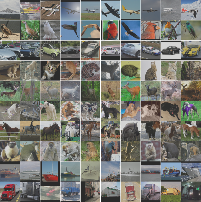
In this blog, we will use CIFAR10 dataset, define a CNN model then train the model and finally test the model on the test data.

Import Libraries

import torch
import torchvision
import torchvision.transforms as transforms

torchvision.__version__

'0.9.1+cu102'

Load the CIFAR10 dataset

Create a transform the images

The output of torchvision datasets are PILImage images of range [0, 1]. We transform them to Tensors of normalized range [-1, 1].

transform = transforms.Compose(
    [transforms.ToTensor(),
     transforms.Normalize((0.5, 0.5, 0.5), (0.5, 0.5, 0.5))])

Load the data and create data loader

batch_size = 5

train_data = torchvision.datasets.CIFAR10(root='./data', train=True,
                                        download=True, transform=transform)

train_data_loader = torch.utils.data.DataLoader(train_data, batch_size=batch_size,
                                          shuffle=True, num_workers=2)

Files already downloaded and verified

test_data = torchvision.datasets.CIFAR10(root='./data', train=False,
                                       download=True, transform=transform)

test_data_loader = torch.utils.data.DataLoader(test_data, batch_size=batch_size,
                                         shuffle=False, num_workers=2)

Files already downloaded and verified

Create the list of classes

class_names = ['plane', 'car', 'bird', 'cat', 'deer', 'dog', 'frog', 'horse', 'ship', 'truck']

Iterate and view the train_data_loader

sample = next(iter(train_data_loader))

imgs, lbls = sample

print(lbls)

tensor([9, 0, 8, 1, 8])

Visualize the train dataset

import matplotlib.pyplot as plt
import numpy as np

def imshow(img):
    img = img / 2 + 0.5     # unnormalize
    npimg = img.numpy()
    
    plt.imshow(np.transpose(npimg, (1, 2, 0)))
    plt.show()


# get some random training images
#dataiter = iter(train_data_loader)
images, labels = iter(train_data_loader).next()

# show images
imshow(torchvision.utils.make_grid(images))
# print labels
print(' '.join(f'{class_names[labels[j]]:5s}' for j in range(batch_size)))

deer  frog  cat   plane car  

Define a Convolutional Neural Network

import torch.nn as nn
import torch.nn.functional as F

class

torch.nn.Conv2d(in_channels, out_channels, kernel_size, stride=1, padding=0, dilation=1, groups=1, bias=True, padding_mode='zeros', device=None, dtype=None): Applies a 2D convolution over an input signal composed of several input planes.

Parameters

in_channels (int) – Number of channels in the input image

out_channels (int) – Number of channels produced by the convolution

kernel_size (int or tuple) – Size of the convolving kernel

stride (int or tuple, optional) – Stride of the convolution. Default: 1

padding (int, tuple or str, optional) – Padding added to all four sides of the input. Default: 0

padding_mode (string, optional) – 'zeros', 'reflect', 'replicate' or 'circular'. Default: 'zeros'

dilation (int or tuple, optional) – Spacing between kernel elements. Default: 1

groups (int, optional) – Number of blocked connections from input channels to output channels. Default: 1

bias (bool, optional) – If True, adds a learnable bias to the output. Default: True

class MyModel(nn.Module):
    def __init__(self):
        super().__init__()
        self.conv1 = nn.Conv2d(3, 6, 5)
        self.pool = nn.MaxPool2d(2, 2)
        self.conv2 = nn.Conv2d(6, 16, 5)
        self.fc1 = nn.Linear(16 * 5 * 5, 120)
        self.fc2 = nn.Linear(120, 84)
        self.fc3 = nn.Linear(84, 10)

    def forward(self, x):
        x = self.pool(F.relu(self.conv1(x)))
        x = self.pool(F.relu(self.conv2(x)))
        x = torch.flatten(x, 1) # flatten all dimensions except batch
        x = F.relu(self.fc1(x))
        x = F.relu(self.fc2(x))
        x = self.fc3(x)
        return x


model = MyModel()

Define a Loss function and optimizer

import torch.optim as optim

loss_function = nn.CrossEntropyLoss()
optimizer = optim.SGD(model.parameters(), lr=0.001, momentum=0.9)

Train the network

for epoch in range(2):  # loop over the dataset multiple times

    running_loss = 0.0
    for i, data in enumerate(train_data_loader, 0):
        # get the inputs; data is a list of [inputs, labels]
        inputs, labels = data

        # zero the parameter gradients
        optimizer.zero_grad()

        # forward + backward + optimize
        outputs = model(inputs)
        loss = loss_function(outputs, labels)
        loss.backward()
        optimizer.step()

        # print statistics
        running_loss += loss.item()
        if i % 2000 == 1999:    # print every 2000 mini-batches
            print(f'[{epoch + 1}, {i + 1:5d}] loss: {running_loss / 2000:.3f}')
            running_loss = 0.0

print('Finished Training')

[1,  2000] loss: 2.196
[1,  4000] loss: 1.893
[1,  6000] loss: 1.653
[1,  8000] loss: 1.597
[1, 10000] loss: 1.506
[2,  2000] loss: 1.475
[2,  4000] loss: 1.390
[2,  6000] loss: 1.392
[2,  8000] loss: 1.371
[2, 10000] loss: 1.320
Finished Training

Save the model

PATH = './conv2d_model.sav'
torch.save(model.state_dict(), PATH)

Test the network on the test data

We have trained the network for 2 passes over the training dataset. But we need to check if the network has learnt anything at all.

We will check this by predicting the class label that the neural network outputs, and checking it against the ground-truth. If the prediction is correct, we add the sample to the list of correct predictions.

Okay, first step. Let us display an image from the test set to get familiar.

dataiter = iter(test_data_loader)
images, labels = dataiter.next()

# print images
imshow(torchvision.utils.make_grid(images))
print('GroundTruth: ', ' '.join(f'{class_names[labels[j]]:5s}' for j in range(4)))

GroundTruth:  cat   ship  ship  plane

Load the saved model

trained_model = MyModel()
trained_model.load_state_dict(torch.load(PATH))

<All keys matched successfully>

Predict

outputs = trained_model(images)

The outputs are energies for the 10 classes. The higher the energy for a class, the more the network thinks that the image is of the particular class. So, let’s get the index of the highest energy:

_, predicted = torch.max(outputs, 1)

print('Predicted: ', ' '.join(f'{class_names[predicted[j]]:5s}'
                              for j in range(4)))

Predicted:  cat   ship  ship  plane

Predict whole test dataset

correct = 0
total = 0
# since we're not training, we don't need to calculate the gradients for our outputs
with torch.no_grad():
    for data in test_data_loader:
        
        images, labels = data
        # calculate outputs by running images through the network
        outputs = trained_model(images)
        
        # the class with the highest energy is what we choose as prediction
        _, predicted = torch.max(outputs.data, 1)
        total += labels.size(0)
        correct += (predicted == labels).sum().item()

print(f'Accuracy of the network on the 10000 test images: {100 * correct // total} %')

Accuracy of the network on the 10000 test images: 53 %

Let us see what are the classes that performed well, and the classes that did not perform well

Prepare to count predictions for each class

correct_pred = {class_name: 0 for class_name in class_names}
print(correct_pred)

total_pred = {class_name: 0 for class_name in class_names}
print(total_pred)

{'plane': 0, 'car': 0, 'bird': 0, 'cat': 0, 'deer': 0, 'dog': 0, 'frog': 0, 'horse': 0, 'ship': 0, 'truck': 0}
{'plane': 0, 'car': 0, 'bird': 0, 'cat': 0, 'deer': 0, 'dog': 0, 'frog': 0, 'horse': 0, 'ship': 0, 'truck': 0}

Predict all test data

# again no gradients needed
with torch.no_grad():
    for data in test_data_loader:
        images, labels = data
        outputs = trained_model(images)
        
        #get the maximum of tensor
        _, predictions = torch.max(outputs, 1)
        
        # collect the correct predictions for each class
        for label, prediction in zip(labels, predictions):
            if label == prediction:
                correct_pred[class_names[label]] += 1
                
            total_pred[class_names[label]] += 1
            pass

        pass

    pass

Print correct and total prediction

print(correct_pred)
print(total_pred)

{'plane': 666, 'car': 532, 'bird': 477, 'cat': 288, 'deer': 347, 'dog': 666, 'frog': 608, 'horse': 504, 'ship': 636, 'truck': 608}
{'plane': 1000, 'car': 1000, 'bird': 1000, 'cat': 1000, 'deer': 1000, 'dog': 1000, 'frog': 1000, 'horse': 1000, 'ship': 1000, 'truck': 1000}

Print accuracy for each class

for class_name, correct_count in correct_pred.items():
    accuracy = 100 * float(correct_count) / total_pred[class_name]
    print(f'Accuracy for class: {class_name:5s} is {accuracy:.1f} %')
    pass

Accuracy for class: plane is 66.6 %
Accuracy for class: car   is 53.2 %
Accuracy for class: bird  is 47.7 %
Accuracy for class: cat   is 28.8 %
Accuracy for class: deer  is 34.7 %
Accuracy for class: dog   is 66.6 %
Accuracy for class: frog  is 60.8 %
Accuracy for class: horse is 50.4 %
Accuracy for class: ship  is 63.6 %
Accuracy for class: truck is 60.8 %